For better or for worse, science has long been married to mathematics. Generally it has been for the better. Especially since the days of Galileo and Newton, math has nurtured science. Rigorous mathematical methods have secured science’s fidelity to fact and conferred a timeless reliability to its findings.
During the past century, though, a mutant form of math has deflected science’s heart from the modes of calculation that had long served so faithfully. Science was seduced by statistics, the math rooted in the same principles that guarantee profits for Las Vegas casinos. Supposedly, the proper use of statistics makes relying on scientific results a safe bet. But in practice, widespread misuse of statistical methods makes science more like a crapshoot.
It’s science’s dirtiest secret: The “scientific method” of testing hypotheses by statistical analysis stands on a flimsy foundation. Statistical tests are supposed to guide scientists in judging whether an experimental result reflects some real effect or is merely a random fluke, but the standard methods mix mutually inconsistent philosophies and offer no meaningful basis for making such decisions. Even when performed correctly, statistical tests are widely misunderstood and frequently misinterpreted. As a result, countless conclusions in the scientific literature are erroneous, and tests of medical dangers or treatments are often contradictory and confusing.
Replicating a result helps establish its validity more securely, but the common tactic of combining numerous studies into one analysis, while sound in principle, is seldom conducted properly in practice.
Experts in the math of probability and statistics are well aware of these problems and have for decades expressed concern about them in major journals. Over the years, hundreds of published papers have warned that science’s love affair with statistics has spawned countless illegitimate findings. In fact, if you believe what you read in the scientific literature, you shouldn’t believe what you read in the scientific literature.
“There is increasing concern,” declared epidemiologist John Ioannidis in a highly cited 2005 paper in PLoS Medicine, “that in modern research, false findings may be the majority or even the vast majority of published research claims.”
Ioannidis claimed to prove that more than half of published findings are false, but his analysis came under fire for statistical shortcomings of its own. “It may be true, but he didn’t prove it,” says biostatistician Steven Goodman of the Johns Hopkins University School of Public Health. On the other hand, says Goodman, the basic message stands. “There are more false claims made in the medical literature than anybody appreciates,” he says. “There’s no question about that.”
Nobody contends that all of science is wrong, or that it hasn’t compiled an impressive array of truths about the natural world. Still, any single scientific study alone is quite likely to be incorrect, thanks largely to the fact that the standard statistical system for drawing conclusions is, in essence, illogical. “A lot of scientists don’t understand statistics,” says Goodman. “And they don’t understand statistics because the statistics don’t make sense.”
Statistical insignificance
Nowhere are the problems with statistics more blatant than in studies of genetic influences on disease. In 2007, for instance, researchers combing the medical literature found numerous studies linking a total of 85 genetic variants in 70 different genes to acute coronary syndrome, a cluster of heart problems. When the researchers compared genetic tests of 811 patients that had the syndrome with a group of 650 (matched for sex and age) that didn’t, only one of the suspect gene variants turned up substantially more often in those with the syndrome — a number to be expected by chance.
“Our null results provide no support for the hypothesis that any of the 85 genetic variants tested is a susceptibility factor” for the syndrome, the researchers reported in the Journal of the American Medical Association.
How could so many studies be wrong? Because their conclusions relied on “statistical significance,” a concept at the heart of the mathematical analysis of modern scientific experiments.
Statistical significance is a phrase that every science graduate student learns, but few comprehend. While its origins stretch back at least to the 19th century, the modern notion was pioneered by the mathematician Ronald A. Fisher in the 1920s. His original interest was agriculture. He sought a test of whether variation in crop yields was due to some specific intervention (say, fertilizer) or merely reflected random factors beyond experimental control.
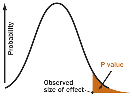
Fisher first assumed that fertilizer caused no difference — the “no effect” or “null” hypothesis. He then calculated a number called the P value, the probability that an observed yield in a fertilized field would occur if fertilizer had no real effect. If P is less than .05 — meaning the chance of a fluke is less than 5 percent — the result should be declared “statistically significant,” Fisher arbitrarily declared, and the no effect hypothesis should be rejected, supposedly confirming that fertilizer works.
Fisher’s P value eventually became the ultimate arbiter of credibility for science results of all sorts — whether testing the health effects of pollutants, the curative powers of new drugs or the effect of genes on behavior. In various forms, testing for statistical significance pervades most of scientific and medical research to this day.
But in fact, there’s no logical basis for using a P value from a single study to draw any conclusion. If the chance of a fluke is less than 5 percent, two possible conclusions remain: There is a real effect, or the result is an improbable fluke. Fisher’s method offers no way to know which is which. On the other hand, if a study finds no statistically significant effect, that doesn’t prove anything, either. Perhaps the effect doesn’t exist, or maybe the statistical test wasn’t powerful enough to detect a small but real effect.
“That test itself is neither necessary nor sufficient for proving a scientific result,” asserts Stephen Ziliak, an economic historian at Roosevelt University in Chicago.
Soon after Fisher established his system of statistical significance, it was attacked by other mathematicians, notably Egon Pearson and Jerzy Neyman. Rather than testing a null hypothesis, they argued, it made more sense to test competing hypotheses against one another. That approach also produces a P value, which is used to gauge the likelihood of a “false positive” — concluding an effect is real when it actually isn’t. What eventually emerged was a hybrid mix of the mutually inconsistent Fisher and Neyman-Pearson approaches, which has rendered interpretations of standard statistics muddled at best and simply erroneous at worst. As a result, most scientists are confused about the meaning of a P value or how to interpret it. “It’s almost never, ever, ever stated correctly, what it means,” says Goodman.
Correctly phrased, experimental data yielding a P value of .05 means that there is only a 5 percent chance of obtaining the observed (or more extreme) result if no real effect exists (that is, if the no-difference hypothesis is correct). But many explanations mangle the subtleties in that definition. A recent popular book on issues involving science, for example, states a commonly held misperception about the meaning of statistical significance at the .05 level: “This means that it is 95 percent certain that the observed difference between groups, or sets of samples, is real and could not have arisen by chance.”
That interpretation commits an egregious logical error (technical term: “transposed conditional”): confusing the odds of getting a result (if a hypothesis is true) with the odds favoring the hypothesis if you observe that result. A well-fed dog may seldom bark, but observing the rare bark does not imply that the dog is hungry. A dog may bark 5 percent of the time even if it is well-fed all of the time. (See Box 2)
Another common error equates statistical significance to “significance” in the ordinary use of the word. Because of the way statistical formulas work, a study with a very large sample can detect “statistical significance” for a small effect that is meaningless in practical terms. A new drug may be statistically better than an old drug, but for every thousand people you treat you might get just one or two additional cures — not clinically significant. Similarly, when studies claim that a chemical causes a “significantly increased risk of cancer,” they often mean that it is just statistically significant, possibly posing only a tiny absolute increase in risk.
Statisticians perpetually caution against mistaking statistical significance for practical importance, but scientific papers commit that error often. Ziliak studied journals from various fields — psychology, medicine and economics among others — and reported frequent disregard for the distinction.
“I found that eight or nine of every 10 articles published in the leading journals make the fatal substitution” of equating statistical significance to importance, he said in an interview. Ziliak’s data are documented in the 2008 book The Cult of Statistical Significance, coauthored with Deirdre McCloskey of the University of Illinois at Chicago.
Multiplicity of mistakes
Even when “significance” is properly defined and P values are carefully calculated, statistical inference is plagued by many other problems. Chief among them is the “multiplicity” issue — the testing of many hypotheses simultaneously. When several drugs are tested at once, or a single drug is tested on several groups, chances of getting a statistically significant but false result rise rapidly. Experiments on altered gene activity in diseases may test 20,000 genes at once, for instance. Using a P value of .05, such studies could find 1,000 genes that appear to differ even if none are actually involved in the disease. Setting a higher threshold of statistical significance will eliminate some of those flukes, but only at the cost of eliminating truly changed genes from the list. In metabolic diseases such as diabetes, for example, many genes truly differ in activity, but the changes are so small that statistical tests will dismiss most as mere fluctuations. Of hundreds of genes that misbehave, standard stats might identify only one or two. Altering the threshold to nab 80 percent of the true culprits might produce a list of 13,000 genes — of which over 12,000 are actually innocent.
Recognizing these problems, some researchers now calculate a “false discovery rate” to warn of flukes disguised as real effects. And genetics researchers have begun using “genome-wide association studies” that attempt to ameliorate the multiplicity issue (SN: 6/21/08, p. 20).
Many researchers now also commonly report results with confidence intervals, similar to the margins of error reported in opinion polls. Such intervals, usually given as a range that should include the actual value with 95 percent confidence, do convey a better sense of how precise a finding is. But the 95 percent confidence calculation is based on the same math as the .05 P value and so still shares some of its problems.
Clinical trials and errors
Statistical problems also afflict the “gold standard” for medical research, the randomized, controlled clinical trials that test drugs for their ability to cure or their power to harm. Such trials assign patients at random to receive either the substance being tested or a placebo, typically a sugar pill; random selection supposedly guarantees that patients’ personal characteristics won’t bias the choice of who gets the actual treatment. But in practice, selection biases may still occur, Vance Berger and Sherri Weinstein noted in 2004 in ControlledClinical Trials. “Some of the benefits ascribed to randomization, for example that it eliminates all selection bias, can better be described as fantasy than reality,” they wrote.
Randomization also should ensure that unknown differences among individuals are mixed in roughly the same proportions in the groups being tested. But statistics do not guarantee an equal distribution any more than they prohibit 10 heads in a row when flipping a penny. With thousands of clinical trials in progress, some will not be well randomized. And DNA differs at more than a million spots in the human genetic catalog, so even in a single trial differences may not be evenly mixed. In a sufficiently large trial, unrandomized factors may balance out, if some have positive effects and some are negative. (See Box 3) Still, trial results are reported as averages that may obscure individual differences, masking beneficial or harmful effects and possibly leading to approval of drugs that are deadly for some and denial of effective treatment to others.
“Determining the best treatment for a particular patient is fundamentally different from determining which treatment is best on average,” physicians David Kent and Rodney Hayward wrote in American Scientist in 2007. “Reporting a single number gives the misleading impression that the treatment-effect is a property of the drug rather than of the interaction between the drug and the complex risk-benefit profile of a particular group of patients.”
Another concern is the common strategy of combining results from many trials into a single “meta-analysis,” a study of studies. In a single trial with relatively few participants, statistical tests may not detect small but real and possibly important effects. In principle, combining smaller studies to create a larger sample would allow the tests to detect such small effects. But statistical techniques for doing so are valid only if certain criteria are met. For one thing, all the studies conducted on the drug must be included — published and unpublished. And all the studies should have been performed in a similar way, using the same protocols, definitions, types of patients and doses. When combining studies with differences, it is necessary first to show that those differences would not affect the analysis, Goodman notes, but that seldom happens. “That’s not a formal part of most meta-analyses,” he says.
Meta-analyses have produced many controversial conclusions. Common claims that antidepressants work no better than placebos, for example, are based on meta-analyses that do not conform to the criteria that would confer validity. Similar problems afflicted a 2007 meta-analysis, published in the New England Journal of Medicine, that attributed increased heart attack risk to the diabetes drug Avandia. Raw data from the combined trials showed that only 55 people in 10,000 had heart attacks when using Avandia, compared with 59 people per 10,000 in comparison groups. But after a series of statistical manipulations, Avandia appeared to confer an increased risk.
In principle, a proper statistical analysis can suggest an actual risk even though the raw numbers show a benefit. But in this case the criteria justifying such statistical manipulations were not met. In some of the trials, Avandia was given along with other drugs. Sometimes the non-Avandia group got placebo pills, while in other trials that group received another drug. And there were no common definitions.
“Across the trials, there was no standard method for identifying or validating outcomes; events … may have been missed or misclassified,” Bruce Psaty and Curt Furberg wrote in an editorial accompanying the New England Journal report. “A few events either way might have changed the findings.”
More recently, epidemiologist Charles Hennekens and biostatistician David DeMets have pointed out that combining small studies in a meta-analysis is not a good substitute for a single trial sufficiently large to test a given question. “Meta-analyses can reduce the role of chance in the interpretation but may introduce bias and confounding,” Hennekens and DeMets write in the Dec. 2 Journal of the American Medical Association. “Such results should be considered more as hypothesis formulating than as hypothesis testing.”
These concerns do not make clinical trials worthless, nor do they render science impotent. Some studies show dramatic effects that don’t require sophisticated statistics to interpret. If the P value is 0.0001 — a hundredth of a percent chance of a fluke — that is strong evidence, Goodman points out. Besides, most well-accepted science is based not on any single study, but on studies that have been confirmed by repetition. Any one result may be likely to be wrong, but confidence rises quickly if that result is independently replicated.
“Replication is vital,” says statistician Juliet Shaffer, a lecturer emeritus at the University of California, Berkeley. And in medicine, she says, the need for replication is widely recognized. “But in the social sciences and behavioral sciences, replication is not common,” she noted in San Diego in February at the annual meeting of the American Association for the Advancement of Science. “This is a sad situation.”
Bayes watch
Such sad statistical situations suggest that the marriage of science and math may be desperately in need of counseling. Perhaps it could be provided by the Rev. Thomas Bayes.
Most critics of standard statistics advocate the Bayesian approach to statistical reasoning, a methodology that derives from a theorem credited to Bayes, an 18th century English clergyman. His approach uses similar math, but requires the added twist of a “prior probability” — in essence, an informed guess about the expected probability of something in advance of the study. Often this prior probability is more than a mere guess — it could be based, for instance, on previous studies.
Bayesian math seems baffling at first, even to many scientists, but it basically just reflects the need to include previous knowledge when drawing conclusions from new observations. To infer the odds that a barking dog is hungry, for instance, it is not enough to know how often the dog barks when well-fed. You also need to know how often it eats — in order to calculate the prior probability of being hungry. Bayesian math combines a prior probability with observed data to produce an estimate of the likelihood of the hunger hypothesis. “A scientific hypothesis cannot be properly assessed solely by reference to the observational data,” but only by viewing the data in light of prior belief in the hypothesis, wrote George Diamond and Sanjay Kaul of UCLA’s School of Medicine in 2004 in the Journal of the American College of Cardiology. “Bayes’ theorem is … a logically consistent, mathematically valid, and intuitive way to draw inferences about the hypothesis.” (See Box 4)
With the increasing availability of computer power to perform its complex calculations, the Bayesian approach has become more widely applied in medicine and other fields in recent years. In many real-life contexts, Bayesian methods do produce the best answers to important questions. In medical diagnoses, for instance, the likelihood that a test for a disease is correct depends on the prevalence of the disease in the population, a factor that Bayesian math would take into account.
But Bayesian methods introduce a confusion into the actual meaning of the mathematical concept of “probability” in the real world. Standard or “frequentist” statistics treat probabilities as objective realities; Bayesians treat probabilities as “degrees of belief” based in part on a personal assessment or subjective decision about what to include in the calculation. That’s a tough placebo to swallow for scientists wedded to the “objective” ideal of standard statistics. “Subjective prior beliefs are anathema to the frequentist, who relies instead on a series of ad hoc algorithms that maintain the facade of scientific objectivity,” Diamond and Kaul wrote.
Conflict between frequentists and Bayesians has been ongoing for two centuries. So science’s marriage to mathematics seems to entail some irreconcilable differences. Whether the future holds a fruitful reconciliation or an ugly separation may depend on forging a shared understanding of probability.
“What does probability mean in real life?” the statistician David Salsburg asked in his 2001 book The Lady Tasting Tea. “This problem is still unsolved, and … if it remains unsolved, the whole of the statistical approach to science may come crashing down from the weight of its own inconsistencies.”
_______________________________________________________________________
BOX 1: Statistics Can Confuse
Statistical significance is not always statistically significant.
It is common practice to test the effectiveness (or dangers) of a drug by comparing it to a placebo or sham treatment that should have no effect at all. Using statistical methods to compare the results, researchers try to judge whether the real treatment’s effect was greater than the fake treatments by an amount unlikely to occur by chance.
By convention, a result expected to occur less than 5 percent of the time is considered “statistically significant.” So if Drug X outperformed a placebo by an amount that would be expected by chance only 4 percent of the time, most researchers would conclude that Drug X really works (or at least, that there is evidence favoring the conclusion that it works).
Now suppose Drug Y also outperformed the placebo, but by an amount that would be expected by chance 6 percent of the time. In that case, conventional analysis would say that such an effect lacked statistical significance and that there was insufficient evidence to conclude that Drug Y worked.
If both drugs were tested on the same disease, though, a conundrum arises. For even though Drug X appeared to work at a statistically significant level and Drug Y did not, the difference between the performance of Drug A and Drug B might very well NOT be statistically significant. Had they been tested against each other, rather than separately against placebos, there may have been no statistical evidence to suggest that one was better than the other (even if their cure rates had been precisely the same as in the separate tests).
“Comparisons of the sort, ‘X is statistically significant but Y is not,’ can be misleading,” statisticians Andrew Gelman of Columbia University and Hal Stern of the University of California, Irvine, noted in an article discussing this issue in 2006 in the American Statistician. “Students and practitioners [should] be made more aware that the difference between ‘significant’ and ‘not significant’ is not itself statistically significant.”
A similar real-life example arises in studies suggesting that children and adolescents taking antidepressants face an increased risk of suicidal thoughts or behavior. Most such studies show no statistically significant increase in such risk, but some show a small (possibly due to chance) excess of suicidal behavior in groups receiving the drug rather than a placebo. One set of such studies, for instance, found that with the antidepressant Paxil, trials recorded more than twice the rate of suicidal incidents for participants given the drug compared with those given the placebo. For another antidepressant, Prozac, trials found fewer suicidal incidents with the drug than with the placebo. So it appeared that Paxil might be more dangerous than Prozac.
But actually, the rate of suicidal incidents was higher with Prozac than with Paxil. The apparent safety advantage of Prozac was due not to the behavior of kids on the drug, but to kids on placebo — in the Paxil trials, fewer kids on placebo reported incidents than those on placebo in the Prozac trials. So the original evidence for showing a possible danger signal from Paxil but not from Prozac was based on data from people in two placebo groups, none of whom received either drug. Consequently it can be misleading to use statistical significance results alone when comparing the benefits (or dangers) of two drugs.
_______________________________________________________________________
A common misinterpretation of the statistician’s P value is that it measures how likely it is that a null (or “no effect”) hypothesis is correct. Actually, the P value gives the probability of observing a result if the null hypothesis is true, and there is no real effect of a treatment or difference between groups being tested. A P value of .05, for instance, means that there is only a 5 percent chance of getting the observed results if the null hypothesis is correct.
It is incorrect, however, to transpose that finding into a 95 percent probability that the null hypothesis is false. “The P value is calculated under the assumption that the null hypothesis is true,” writes biostatistician Steven Goodman. “It therefore cannot simultaneously be a probability that the null hypothesis is false.”
Consider this simplified example. Suppose a certain dog is known to bark constantly when hungry. But when well-fed, the dog barks less than 5 percent of the time. So if you assume for the null hypothesis that the dog is not hungry, the probability of observing the dog barking (given that hypothesis) is less than 5 percent. If you then actually do observe the dog barking, what is the likelihood that the null hypothesis is incorrect and the dog is in fact hungry?
Answer: That probability cannot be computed with the information given. The dog barks 100 percent of the time when hungry, and less than 5 percent of the time when not hungry. To compute the likelihood of hunger, you need to know how often the dog is fed, information not provided by the mere observation of barking.
_______________________________________________________________________
BOX 3: Randomness and Clinical Trials
Assigning patients at random to treatment and control groups is an essential feature of controlled clinical trials, but statistically that approach cannot guarantee that individual differences among patients will always be distributed equally. Experts in clinical trial analyses are aware that such incomplete randomization will leave some important differences unbalanced between experimental groups, at least some of the time.
“This is an important concern,” says biostatistician Don Berry of M.D. Anderson Cancer Center in Houston.
In an e-mail message, Berry points out that two patients who appear to be alike may respond differently to identical treatments. So statisticians attempt to incorporate patient variability into their mathematical models.
“There may be a googol of patient characteristics and it’s guaranteed that not all of them will be balanced by randomization,” Berry notes. “But some characteristics will be biased in favor of treatment A and others in favor of treatment B. They tend to even out. What is not evened out is regarded by statisticians to be ‘random error,’ and this we model explicitly.”
Understanding the individual differences affecting response to treatment is a major goal of scientists pursuing “personalized medicine,” in which therapies are tailored to each person’s particular biology. But the limits of statistical methods in drawing conclusions about subgroups of patients pose a challenge to achieving that goal.
“False-positive observations abound,” Berry acknowledges. “There are patients whose tumors melt away when given some of our newer treatments.… But just which one of the googol of characteristics of this particular tumor enabled such a thing? It’s like looking for a needle in a haystack … or rather, looking for one special needle in a stack of other needles.”
_______________________________________________________________________
Bayesian methods of statistical analysis stem from a paper published posthumously in 1763 by the English clergyman Thomas Bayes. In a Bayesian analysis, probability calculations require a prior value for the likelihood of an association, which is then modified after data are collected. When the prior probability isn’t known, it must be estimated, leading to criticisms that subjective guesses must often be incorporated into what ought to be an objective scientific analysis. But without such an estimate, statistics can produce grossly inaccurate conclusions.
For a simplified example, consider the use of drug tests to detect cheaters in sports. Suppose the test for steroid use among baseball players is 95 percent accurate — that is, it correctly identifies actual steroid users 95 percent of the time, and misidentifies non-users as users 5 percent of the time.
Suppose an anonymous player tests positive. What is the probability that he really is using steroids? Since the test really is accurate 95 percent of the time, the naïve answer would be that probability of guilt is 95 percent. But a Bayesian knows that such a conclusion cannot be drawn from the test alone. You would need to know some additional facts not included in this evidence. In this case, you need to know how many baseball players use steroids to begin with — that would be what a Bayesian would call the prior probability.
Now suppose, based on previous testing, that experts have established that about 5 percent of professional baseball players use steroids. Now suppose you test 400 players. How many would test positive?
• Out of the 400 players, 20 are users (5 percent) and 380 are not users.
• Of the 20 users, 19 (95 percent) would be identified correctly as users.
• Of the 380 nonusers, 19 (5 percent) would incorrectly be indicated as users.
So if you tested 400 players, 38 would test positive. Of those, 19 would be guilty users and 19 would be innocent nonusers. So if any single player’s test is positive, the chances that he really is a user are 50 percent, since an equal number of users and nonusers test positive.